In this article, we will discuss some of the top libraries in Python that can be used by developers to prase, clean, and represent data and implement machine learning in their existing applications.
We will be considering the following 10 libraries:
- TensorFlow
- Scikit-Learn
- Numpy
- Keras
- PyTorch
- LightGBM
- Eli5
- SciPy
- Theano
- Pandas

Introduction
Python is one of the most popular and widely used programming languages and has replaced many programming languages in the industry.
There are many reasons why Python is popular among developers. However, one of the most significant is its large collection of libraries that users can work with.
The simplicity of Python has attracted many developers to create new libraries for machine learning. Because of the huge collection of libraries, Python is becoming hugely popular among machine learning experts.
So, the first library is TensorFlow.
TensorFlow
![]()
What Is TensorFlow?
If you are currently working on a machine learning project in Python, then you may have heard about this popular open-source library known as TensorFlow.
This library was developed by Google in collaboration with the Brain Team. TensorFlow is used in almost every Google application for machine learning.
TensorFlow works like a computational library for writing new algorithms that involve a large number of tensor operations. Since neural networks can be easily expressed as computational graphs, they can be implemented using TensorFlow as a series of operations on Tensors. Plus, tensors are N-dimensional matrices that represent your data.
Features of TensorFlow
TensorFlow is optimized for speed, and it makes use of techniques like XLA for quick linear algebra operations.
1. Responsive Construct
With TensorFlow, we can easily visualize each and every part of the graph, which is not an option while using Numpy or SciKit.
2. Flexible
One of the very important Tensorflow Features is that it is flexible in its operability, meaning it has modularity, and for the parts of it that you want to make stand alone, it offers you that option.
3. Easily Trainable
It is easily trainable on CPU as well as GPU for distributed computing.
4. Parallel Neural Network Training
TensorFlow offers pipelining, in the sense that you can train multiple neural networks and multiple GPUs, which makes the models very efficient on large-scale systems.
5. Large Community
Needless to say, if it has been developed by Google, there is already a large team of software engineers who work on stability improvements continuously.
6. Open Source
The best thing about this machine learning library is that it is open source, so anyone can use it as long as they have internet connectivity.
Where Is TensorFlow Used?
You are using TensorFlow daily but indirectly with applications like Google Voice Search or Google Photos. These applications are developed using this library.
All the libraries created in TensorFlow are written in C and C++. However, it has a complicated frontend for Python. Your Python code will get compiled and then executed on TensorFlow distributed execution engine built using C and C++.
The number of applications of TensorFlow is literally unlimited, and that is the beauty of TensorFlow.
Scikit-Learn
What Is Scikit-learn?
It is a Python library is associated with NumPy and SciPy. It is considered one of the best libraries for working with complex data.
There are a lot of changes being made in this library. One modification is the cross-validation feature, providing the ability to use more than one metric. Lots of training methods like logistics regression and nearest neighbors have received some little improvements.
Features Of Scikit-Learn
1. Cross-validation: There are various methods to check the accuracy of supervised models on unseen data.
2.Unsupervised learning algorithms: Again, there is a large spread of algorithms in the offering — starting from clustering, factor analysis, and principal component analysis to unsupervised neural networks.
3. Feature extraction: Useful for extracting features from images and text (e.g. Bag of words
Where Is Scikit-Learn Used?
It contains a numerous number of algorithms for implementing standard machine learning and data mining tasks like reducing dimensionality, classification, regression, clustering, and model selection.
Numpy
![]()
What Is Numpy?
Numpy is considered one of the most popular machine learning libraries in Python.
TensorFlow and other libraries use Numpy internally for performing multiple operations on Tensors. Array interface is the best and the most important feature of Numpy.
Features Of Numpy
- Interactive: Numpy is very interactive and easy to use
- Mathematics: Makes complex mathematical implementations very simple
- Intuitive: Makes coding real easy and grasping the concepts is easy
- Lots of Interaction: Widely used, hence a lot of open source contribution
Where Is Numpy Used?
This interface can be utilized for expressing images, sound waves, and other binary raw streams as an array of real numbers in N-dimensional.
For implementing this library for machine learning, having knowledge of Numpy is important for full-stack developers.
Keras
![]()
What Is Keras?
Keras is considered one of the coolest machine learning libraries in Python. It provides an easier mechanism to express neural networks. Keras also provides some of the best utilities for compiling models, processing data-sets, visualization of graphs, and much more.
In the backend, Keras uses either Theano or TensorFlow internally. Some of the most popular neural networks like CNTK can also be used. Keras is comparatively slow when we compare it with other machine learning libraries because it creates a computational graph by using back-end infrastructure and then makes use of it to perform operations. All the models in Keras are portable.
Features Of Keras
- It runs smoothly on both CPU and GPU.
- Keras supports almost all the models of a neural network — fully connected, convolutional, pooling, recurrent, embedding, etc. Furthermore, these models can be combined to build more complex models.
- Keras, being modular in nature, is incredibly expressive, flexible, and apt for innovative research.
- Keras is a completely Python-based framework, which makes it easy to debug and explore.
Where Is Keras Used?
You are already constantly interacting with features built with Keras — it is in use at Netflix, Uber, Yelp, Instacart, Zocdoc, Square, and many others. It is especially popular among startups that place deep learning at the core of their products.
Keras contains numerous implementations of commonly used neural network building blocks such as layers, objectives, activation functions, optimizers and a host of tools to make working with image and text data easier.
Plus, it provides many pre-processed data-sets and pre-trained models like MNIST, VGG, Inception, SqueezeNet, ResNet, etc.
Keras is also a favorite among deep learning researchers, coming in at #2. Keras has also been adopted by researchers at large scientific organizations, in particular, CERN and NASA.
PyTorch
![]()
What Is PyTorch?
PyTorch is the largest machine learning library that allows developers to perform tensor computations with the acceleration of GPU, creates dynamic computational graphs, and calculate gradients automatically. Other than this, PyTorch offers rich APIs for solving application issues related to neural networks.
This machine learning library is based on Torch, which is an open-source machine library implemented in C with a wrapper in Lua.
This machine library, in Python, was introduced in 2017, and since its inception, the library is gaining popularity and attracting an increasing number of machine learning developers.
Features Of PyTorch
Hybrid Front-End
A new hybrid frontend provides ease-of-use and flexibility in eager mode, while seamlessly transitioning to graph mode for speed, optimization, and functionality in C++ runtime environments.
Distributed Training
Optimize performance in both research and production by taking advantage of native support for asynchronous execution of collective operations and peer-to-peer communication that is accessible from Python and C++.
Python First
PyTorch is not a Python binding into a monolithic C++ framework. It’s built to be deeply integrated into Python so it can be used with popular libraries and packages such as Cython and Numba.
Libraries and Tools
An active community of researchers and developers have built a rich ecosystem of tools and libraries for extending PyTorch and supporting development in areas from computer vision to reinforcement learning.
Where Is PyTorch Used?
PyTorch is primarily used for applications such as natural language processing.
It is primarily developed by Facebook’s artificial-intelligence research group and Uber’s “Pyro” software for probabilistic programming is built on it.
PyTorch is outperforming TensorFlow in multiple ways and it is gaining a lot of attention in recent days.
LightGBM
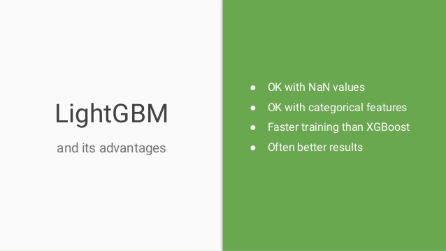
What Is LightGBM?
Gradient Boosting is one of the best and most popular machine learning(ML) library, which helps developers in building new algorithms by using redefined elementary models and namely decision trees. Therefore, there are special libraries that are designed for fast and efficient implementation of this method.
These libraries are LightGBM, XGBoost, and CatBoost. All these libraries are competitors that help in solving a common problem and can be utilized in almost a similar manner.
Features of LightGBM
Very fast computation ensures high production efficiency.
Intuitive, hence makes it user-friendly.
Faster training than many other deep learning libraries.
Will not produce errors when you consider NaN values and other canonical values.
Where Is LightGBM Used?
This library provides highly scalable, optimized, and fast implementations of gradient boosting, which makes it popular among machine learning developers. Because most of the machine learning full-stack developers won machine learning competitions by using these algorithms.
Eli5
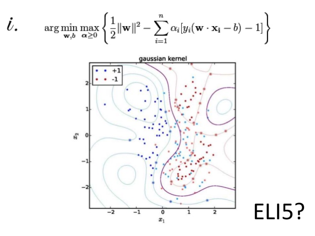
What Is Eli5?
Most often, the results of machine learning model predictions are not accurate, and Eli5 machine learning library built-in Python helps in overcoming this challenge. It is a combination of visualization and debugs all the machine learning models and tracks all working steps of an algorithm.
Features of Eli5
Moreover, Eli5 supports other libraries XGBoost, lightning, scikit-learn, and sklearn-crfsuite libraries. All the above-mentioned libraries can be used to perform different tasks using each one of them.
Where Is Eli5 Used?
- Mathematical applications that require a lot of computation in a short time.
- Eli5 plays a vital role where there are dependencies with other Python packages.
- Legacy applications and implementing newer methodologies in various fields.
SciPy

What Is SciPy?
SciPy is a machine learning library for application developers and engineers. However, you still need to know the difference between SciPy library and SciPy stack. SciPy library contains modules for optimization, linear algebra, integration, and statistics.
Features Of SciPy
The main feature of the SciPy library is that it is developed using NumPy, and its array makes the most use of NumPy.
In addition, SciPy provides all the efficient numerical routines like optimization, numerical integration, and many others using its specific submodules.
All the functions in all submodules of SciPy are well documented.
Where Is SciPy Used?
SciPy is a library that uses NumPy for the purpose of solving mathematical functions. SciPy uses NumPy arrays as the basic data structure and comes with modules for various commonly used tasks in scientific programming.
Tasks including linear algebra, integration (calculus), ordinary differential equation solving and signal processing are handled easily by SciPy.
Theano
![]()
What Is Theano?
Theano is a computational framework machine learning library in Python for computing multidimensional arrays. Theano works similar to TensorFlow, but it not as efficient as TensorFlow. Because of its inability to fit into production environments.
Moreover, Theano can also be used on a distributed or parallel environments just similar to TensorFlow.
Features Of Theano
- Tight integration with NumPy – Ability to use completely NumPy arrays in Theano-compiled functions.
- Transparent use of a GPU – Perform data-intensive computations much faster than on a CPU.
- Efficient symbolic differentiation – Theano does your derivatives for functions with one or many inputs.
- Speed and stability optimizations – Get the right answer for
log(1+x)even whenxis very tiny. This is just one of the examples to show the stability of Theano. - Dynamic C code generation – Evaluate expressions faster than ever before, thereby increasing efficiency by a lot.
- Extensive unit-testing and self-verification – Detect and diagnose multiple types of errors and ambiguities in the model.
Where Is Theano Used?
The actual syntax of Theano expressions is symbolic, which can be off-putting to beginners used to normal software development. Specifically, an expression is defined in the abstract sense, compiled, and later actually used to make calculations.
It was specifically designed to handle the types of computation required for large neural network algorithms used in Deep Learning. It was one of the first libraries of its kind (development started in 2007) and is considered an industry standard for Deep Learning research and development.
Theano is being used in multiple neural network projects today, and the popularity of Theano is only growing with time.
Pandas
What Is Pandas?
Pandas is a machine learning library in Python that provides data structures of high-level and a wide variety of tools for analysis. One of the great features of this library is the ability to translate complex operations with data using one or two commands. Pandas has so many inbuilt methods for grouping, combining data, filtering, as well as time-series functionality.
All these are followed by outstanding speed indicators.
Features Of Pandas
Pandas makes sure that the entire process of manipulating data will be easier. Support for operations such as Re-indexing, Iteration, Sorting, Aggregations, Concatenations, and Visualizations are among the feature highlights of Pandas.
Where Is Pandas Used?
Currently, there are fewer releases of the Pandas library, which includes hundreds of new features, bug fixes, enhancements, and changes in API. The improvements in Pandas are its ability to group and sort data, select the best-suited output for the applied method, and provide support for performing custom types operations.
Data Analysis, among everything else, takes the highlight when it comes to using Pandas. But when used with other libraries and tools, Pandas ensures high functionality and a good amount of flexibility.
That’s it, folks! I hope this article helped you kickstart your learning the libraries available in Python.